Trends

trend computes a Theil–Sen slope and a Mann–Kendall test for every pixel of a time series cube, against the real dates.

import eofigs

result = eofigs.trend(ndvi_cube, per="decade")  # time, y, x -> y, x
result.slope  # NDVI per decade
result.significant  # p < 0.05

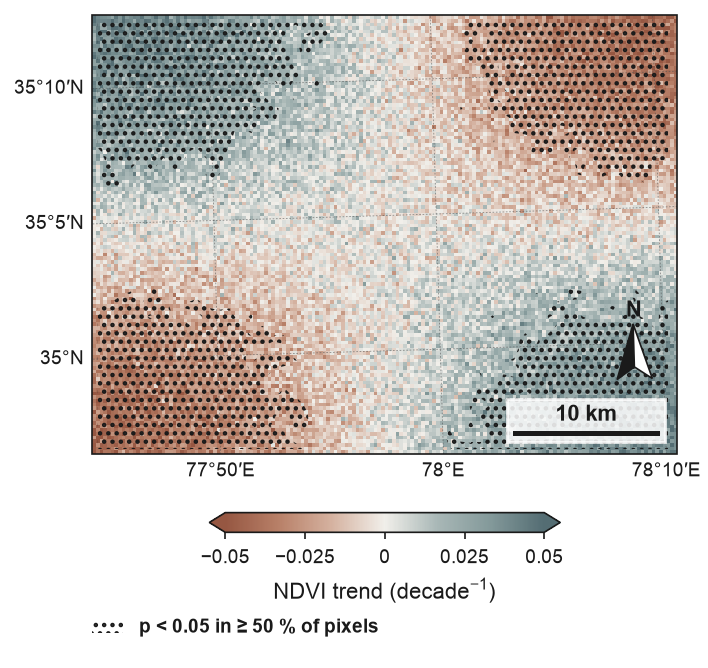
The figure shows a synthetic annual NDVI series (2000–2024) with greening and browning regions and noise, drawn with trend_map: the Theil–Sen slope with the library's vegetation trend colours, and hatching where the Mann–Kendall test gives p < 0.05 for at least half of the pixels in each cell. The full script is on the gallery page.

Output

Variable	Meaning
slope	median of all pairwise slopes, in data units per per ("decade" or "year")
intercept	median of y - slope * t: the value at the first date, stored in its reference_time attribute
pvalue	two-sided Mann–Kendall p-value
significant	pvalue < alpha (default 0.05)
n_valid	number of valid observations

Pixels with fewer than min_valid observations (default 8) are NaN. Spatial coordinates and the CRS are kept, so the result plots directly as a map. The slope is labelled as a trend of the input variable (for NDVI: "Normalized Difference Vegetation Index trend", decade$^{-1}$), so eofigs.variable(result.slope) returns the variable's trend with zero-centred colours.

Method and assumptions

• Time: slopes use the datetime coordinate converted to years, so gaps and irregular steps are handled. A time axis that is not datetime64 raises an error.
• Theil–Sen slope (Sen 1968) and intercept as in scipy.stats.theilslopes(method="joint"); the tests compare both with SciPy for every pixel.
• Mann–Kendall test (Mann 1945; Kendall 1975) with the tie correction of the variance and the continuity correction of Z.
• Assumptions: observations are treated as serially independent; no correction for autocorrelation (modified Mann–Kendall, prewhitening) is applied. For monthly or other sub-annual data use the seasonal test below, or aggregate to annual values first.

Seasonal data

A seasonal cycle distorts the plain Mann–Kendall test and the Theil–Sen slope of monthly data: most pairs of values compare different times of the year. seasonal="month" uses the seasonal Mann–Kendall test and the seasonal Kendall slope (Hirsch et al. 1982) instead: each month is compared only with the same month in other years, and the statistics are summed over the months.

result = eofigs.trend(monthly_ndvi, seasonal="month")  # 12 calendar months
growing = monthly_ndvi.sel(time=monthly_ndvi.time.dt.month.isin([5, 6, 7, 8, 9]))
result = eofigs.trend(growing, seasonal="month")  # May to September only: 5 seasons
result.attrs["seasonal_correction"]  # 'Hirsch-Slack 1984'

• Seasons: "month" (the calendar month of each date), or an array with one label per time step for other periods. For 16- or 8-day composites, label each value by its composite, for example its day of year: seasonal=composites.time.dt.dayofyear.values. Each season may have one value per calendar year; more than one raises an error that names the season and year (resample, for example to monthly means, or use finer labels). Seasons with fewer than 4 values in a pixel are left out of its test, as in the R package rkt.
• Correlation between seasons: values of consecutive months of one year usually move together, which makes the seasonal test too willing to find a trend. By default the variance of the test statistic includes the covariances between seasons (Hirsch and Slack 1984; the same computation as rkt(..., correct = TRUE)). The correction needs at least 10 complete years; with fewer, the uncorrected test is used with a TrendWarning, and trend_map's caption says so. A complete year is a calendar year in which the time axis has a step for every season, so the count is the same for every pixel; gaps within a pixel are handled by mean ranks and by leaving out seasons with fewer than 4 values. seasonal_correction=False treats the seasons as independent.
• Without seasonal, sub-annual data (median step under 300 days) get a TrendWarning suggesting seasonal="month"; seasonal="none" keeps the plain test and states the choice.
• Checked against R: the tests compare S, the variances with and without the correction, the p-values and the slope with trend::smk.test, trend::csmk.test, trend::sea.sens.slope and rkt::rkt (script: docs/scripts/seasonal_mk_reference.R).

The seasonal trend map of Swat monthly NDVI shows the effect of the correction: 59.6 % of the vegetated pixels are significant with it, 63.4 % without.

Hirsch, R. M., Slack, J. R., & Smith, R. A. (1982). Techniques of trend analysis for monthly water quality data. Water Resources Research, 18(1), 107–121. doi:10.1029/WR018i001p00107

Hirsch, R. M., & Slack, J. R. (1984). A nonparametric trend test for seasonal data with serial dependence. Water Resources Research, 20(6), 727–732. doi:10.1029/WR020i006p00727

Memory and time

The pairwise slopes are processed in blocks of pixels that fit memory_mb (default 256 MB), so any series length works. The work grows with the number of pairs, n(n−1)/2, per pixel:

Series	Pixels	One core	dask, 32 threads
300 monthly steps	20 000	37 s	7.6 s
300 monthly steps	1 000 000 (extrapolated)	about 30 min	about 6 min

Peak memory stayed near 400 MB for every size. For large cubes pass a dask-backed array (for example cube.chunk({"x": 500, "y": 500})); the blocks then run in parallel. Annual series are much faster: 25 steps have 300 pairs instead of 44 850. For long monthly series, use the seasonal test (see Seasonal data) or aggregate to annual values.

References

• Sen, P. K. (1968). Estimates of the regression coefficient based on Kendall's tau. Journal of the American Statistical Association, 63, 1379–1389.
• Mann, H. B. (1945). Nonparametric tests against trend. Econometrica, 13, 245–259.
• Kendall, M. G. (1975). Rank Correlation Methods. Griffin, London.