Seasonal trend map: Swat valley monthly NDVI

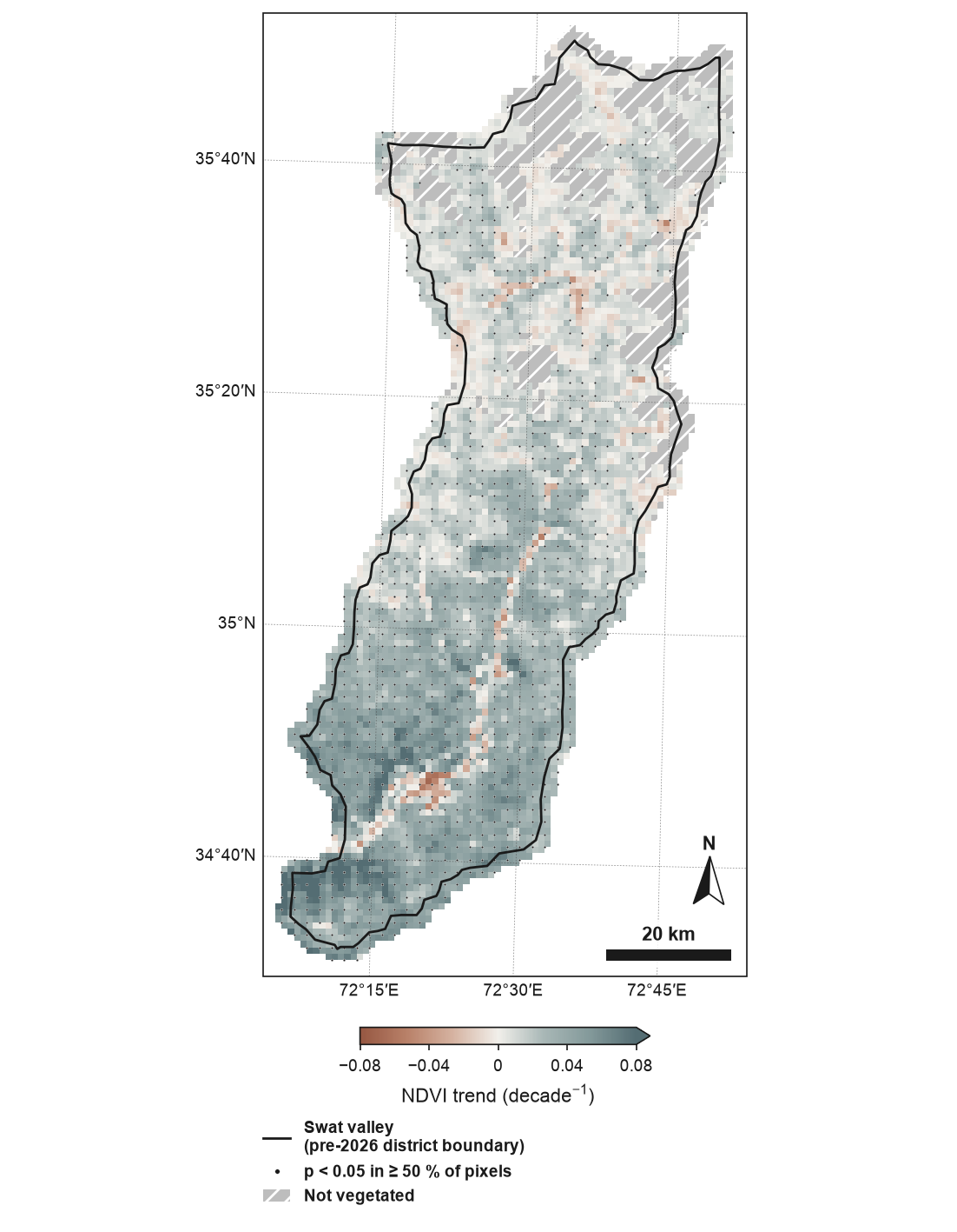
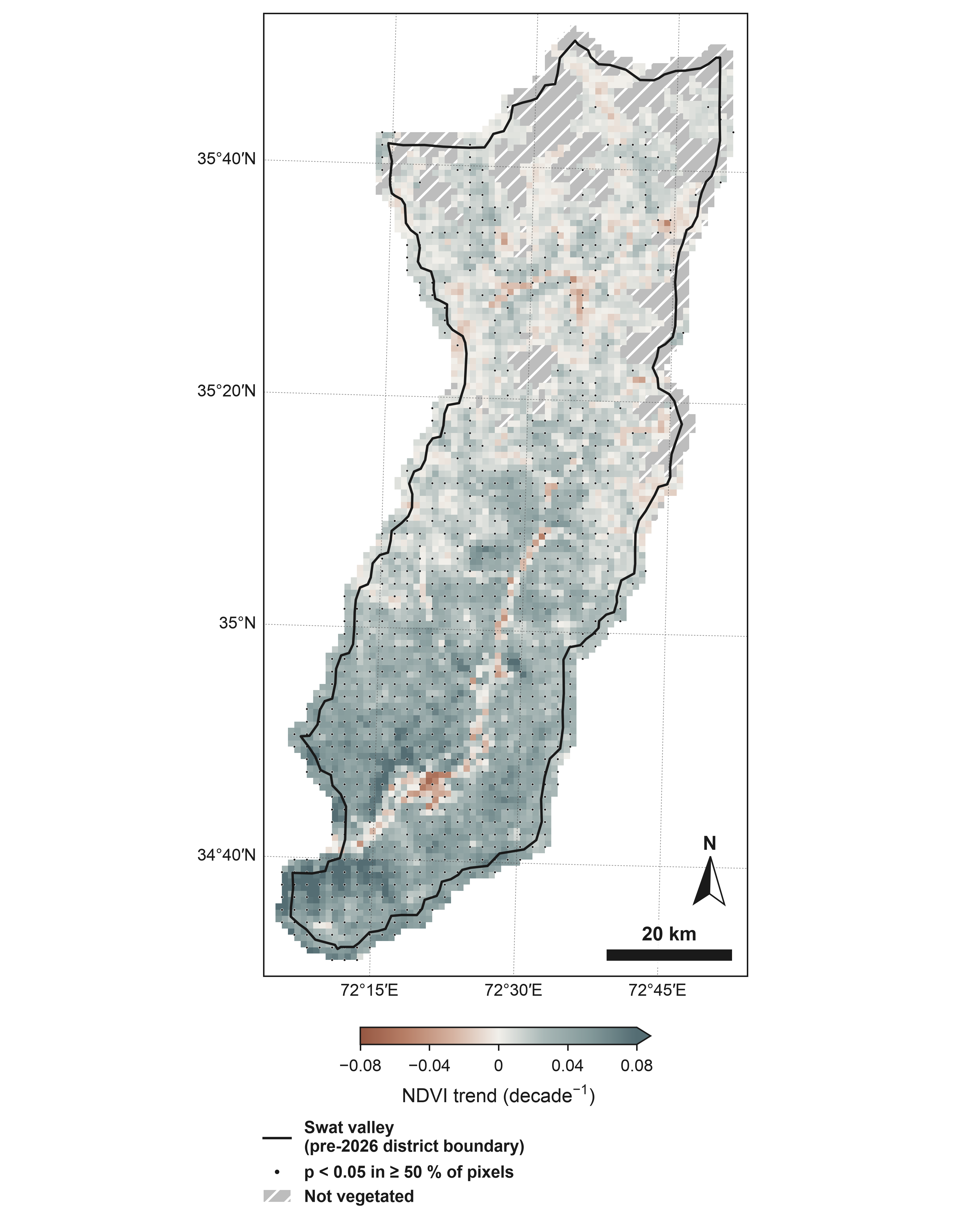
Seasonal Kendall trend of monthly NDVI for May to September (MODIS Terra MOD13A1 v6.1, monthly medians of the 16-day composites, 1 km), 2001–2021, around the Swat valley (pre-2026 district boundary): the former Swat district (before January 2026), now Swat and Bar Swat (geoBoundaries). The test and the slope compare each month only with the same month in other years (seasonal="month", 5 seasons), so the seasonal cycle does not enter them. Dots: at least 50 % of 1000 m pixels significant (seasonal Mann–Kendall with the Hirsch–Slack correction for correlation between seasons, p < 0.05): 59.6 % of the vegetated pixels with a valid trend. Without the correction (seasonal_correction=False) 63.4 % would be marked: consecutive months of one year move together, and treating them as independent makes the test too willing to find a trend. Per-pixel seasonal Mann–Kendall tests assume independence between years and are not adjusted for multiple comparisons. Grey with diagonal hatching: mean NDVI below 0.1 over the record (not vegetated; 13.8 % of the pixels with data). Pixels without data (beyond 2 km outside the outline) are left white. MODIS data: NASA LP DAAC, accessed through the Microsoft Planetary Computer. Boundaries and names shown do not imply any opinion on the legal status of any country or territory.

Script PDF PNG, 600 dpi

from pathlib import Path

import matplotlib.pyplot as plt
import pandas as pd
import rioxarray

import eofigs

DATA = Path(__file__).resolve().parents[1] / "docs" / "data" / "swat"


def swat_monthly_ndvi():
    """Load the monthly NDVI cube (one band per month, named YYYY-MM) with a time axis."""
    raw = rioxarray.open_rasterio(DATA / "swat_ndvi_monthly_1km.tif", mask_and_scale=True)
    months = pd.to_datetime([f"{month}-01" for month in raw.attrs["long_name"]])
    cube = raw.rename(band="time").assign_coords(time=months)
    cube.name = "ndvi"
    cube.attrs = {"long_name": "NDVI", "units": "1"}
    return cube


cube = swat_monthly_ndvi()
growing_season = cube.sel(time=cube.time.dt.month.isin([5, 6, 7, 8, 9]))
outline = {
    "aoi": DATA / "swat_boundary.geojson",
    "aoi_label": "Swat valley\n(pre-2026 district boundary)",
    "width": "onehalf",
}
eofigs.set_style("elsevier")
fig = eofigs.trend_map(growing_season, seasonal="month", **outline)
uncorrected = eofigs.trend_map(growing_season, seasonal="month", seasonal_correction=False,
                               **outline)  # fmt: skip
shares = {
    "with the Hirsch-Slack correction": fig.eofigs_layout["significant_percent"],
    "without it": uncorrected.eofigs_layout["significant_percent"],
}
plt.close(uncorrected)  # drawn only for its record

if __name__ == "__main__":
    print(fig.eofigs_layout["caption"])
    print(shares)
    print(eofigs.save_figure(fig, "seasonal_trend_swat"))

Figure check

Figure check (elsevier): passed
  PASS  size: 140.0 x 180.0 mm (onehalf width).
  PASS  resolution: 600 dpi (at least 500 for figures with text and images).
  PASS  font size: Smallest text 7 pt (minimum 7 pt).
  PASS  fonts: Fonts in use: Arial.
  PASS  colour-blind safety: 3 categorical colours, all distinguishable.
  PASS  colour maps: Colour maps: eofigs.terra_slate (diverging).