Study area maps

study_area_map draws the map most Earth observation papers open with: the study area on relief, with the context a reader needs to place it.

import eofigs

eofigs.set_style("elsevier")
fig = eofigs.study_area_map(
    "swat_boundary.geojson",
    dem="swat_dem_90m.tif",  # hillshade + elevation colours
    overlay="swat_tree_cover_90m.tif",  # drawn where it reaches 50 %
    points="swat_towns.geojson",  # labelled from the "name" column
    aoi_label="Swat valley\n(pre-2026 district boundary)",
    overlay_label="Tree cover ≥ 50 %",
    points_label="Town",
    width="onehalf",
)
eofigs.save_figure(fig, "figures/fig1")

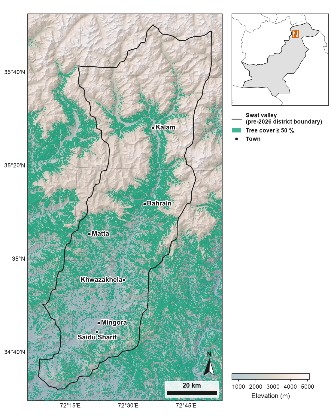
The outline is the former Swat district (before January 2026), now Swat and Bar Swat. Produced using Copernicus WorldDEM™-90 © DLR e.V. 2010-2014 and © Airbus Defence and Space GmbH 2014-2018 provided under COPERNICUS by the European Union and ESA; all rights reserved. © ESA WorldCover project 2021 / Contains modified Copernicus Sentinel data (2021) processed by ESA WorldCover consortium. Towns: GeoNames (CC BY 4.0). Locator inset: Natural Earth. Boundaries and names shown do not imply any opinion on the legal status of any country or territory. Full code and downloads: gallery.

What is on the map

Element	Default
Map CRS	the study area's CRS if projected, otherwise its UTM zone
Study area	black outline, 1 pt
Relief	grey hillshade (azimuth 315°, altitude 45°) under elevation colours at 45 % opacity: batlow, or with an overlay the light, low-chroma half of lapaz so the overlay stands out; a colour bar with four or five round ticks. DEMs are reduced to the printed resolution first, and no-data is grey #BDBDBD
Overlay	one colour (Okabe–Ito bluish green #009E73) at 75 % opacity, so the hillshade shows through, where the raster is True or reaches the threshold (50 for percentages, 0.5 for fractions)
Points	black dots with a white edge; bold labels with a white halo, placed so that they overlap neither each other, the other points nor the outline
Graticule	at most four labelled lines per side, at round degrees or minutes
North arrow	points to true north: rotated by the grid convergence at the map centre (1.4° in the Swat example, which lies west of the UTM zone's central meridian); placed above or beside the scale bar with a 2 mm gap
Scale bar	a round length (1, 2, 2.5 or 5 × 10ⁿ km) near 22 % of the map width, or a shorter round length where that does not fit; true ground distance at the map centre (the projection's scale factor is taken into account)
Locator inset	the surrounding country in grey, neighbours in white, the study area in vermillion

Layout

The figure width is a journal width; the height follows the study area's shape, up to three quarters of the journal's maximum height (pass height_mm for any other height). Two layouts:

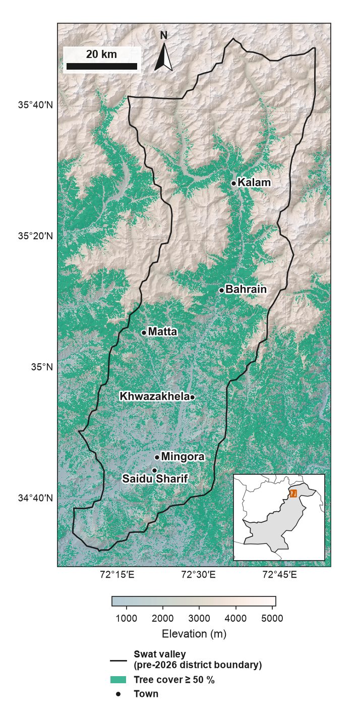
• inside: inset, legend, and north arrow with scale bar sit in the emptiest parts of the map, and the colour bar sits below the map. Items never touch the study area outline (they keep 2 mm from it), the points or their labels, and the inset and legend only go where at least 85 % of the space under them lies outside the study area. A legend that finds no such place goes below the map, beside or under the colour bar.
• side: inset, legend and colour bar sit in a column beside the map; the north arrow and scale bar stay in an empty part of the map, or go to the column when there is none.

layout="auto" (default) uses the side layout for tall study areas at 120 mm or wider, and the inside layout otherwise, switching to the side layout when the inset finds no empty position inside the map. fig.eofigs_layout records what was chosen.

One panel of a larger figure

study_area_map(..., subfigure=sub) draws the map, its legend, inset and colour bar within a matplotlib subfigure, so a map can sit beside a chart in one figure:

fig, ax0 = eofigs.new_figure("double", height_mm=200, layout="none")
ax0.remove()
left, right = fig.subfigures(1, 2, width_ratios=[105, 85])
eofigs.study_area_map("aoi.geojson", dem="dem.tif", subfigure=left)
chart = right.add_axes((0.2, 0.12, 0.72, 0.85))
eofigs.label_panels([left.axes[0], chart])

The house style gallery entry shows a full example.

Overlay colours

check_figure tests that a single-colour overlay stays distinguishable from the semi-transparent colour map under it, as they appear on the page: CIEDE2000 of at least 10 in normal vision and 6 under simulated colour-vision deficiency. Muted sage (#A4B9A8) is too close to batlow's greens (minimum difference about 1), so the default overlay colour is Okabe–Ito bluish green. Strong elevation colours also compete with an overlay, so under one eofigs switches to the light half of lapaz: of the light, low-chroma ranges tested (grayC, bilbao, lapaz), it passes with the widest margin (23.5 in normal vision, 12.9 for protan; grayC and bilbao fall below 6 for deutan or protan).

Boundaries and worldviews

The inset uses Natural Earth's 1:110m countries with de facto boundaries (who administers an area), bundled with eofigs. For disputed areas, Natural Earth also publishes the boundaries as seen by 31 countries ("worldviews"), for example worldview="PAK" or worldview="IND". A worldview is downloaded once (about 5 MB, version 5.1.2, checksum verified), simplified to inset scale and cached; offline, eofigs says so and keeps working with the default. Your own outlines can be passed with inset=<GeoDataFrame>.

Several countries regulate how maps published there show their borders, and journals have their own policies; choose the worldview for the journal and the readership, and add a line such as: Boundaries and names shown do not imply any opinion on the legal status of any country or territory.

Map elements on their own

add_north_arrow(ax), add_scale_bar(ax) and add_inset(ax, aoi) work on any cartopy map, for example in a multi-panel figure.

Sample data

The Swat valley files in docs/data/swat/ (DEM, tree cover, outline, towns) are in the repository but not in the installed package; their licences and the required notices are in DATA_LICENSES.md.