Event composites

event_composite shows how the land surface responded to a set of events (droughts, heatwaves, floods, fires): anomaly maps for the periods before, during and after the events, averaged over the events, and the composite series around the event start.

import eofigs

eofigs.set_style("elsevier")
fig = eofigs.event_composite(
    monthly_ndvi,  # time, y, x with a CRS
    [("2001-05-01", "2001-05-01"), ("2006-05-01", "2006-05-01"), ("2009-08-01", "2009-08-01")],
    event_rule="May–September months with tmax z ≥ +1 and precipitation z ≤ −1",
    aoi="swat_boundary.geojson",
    aoi_label="Swat valley\n(pre-2026 district boundary)",
)
print(fig.eofigs_layout["caption"])  # events, method, limits, significance, masked classes

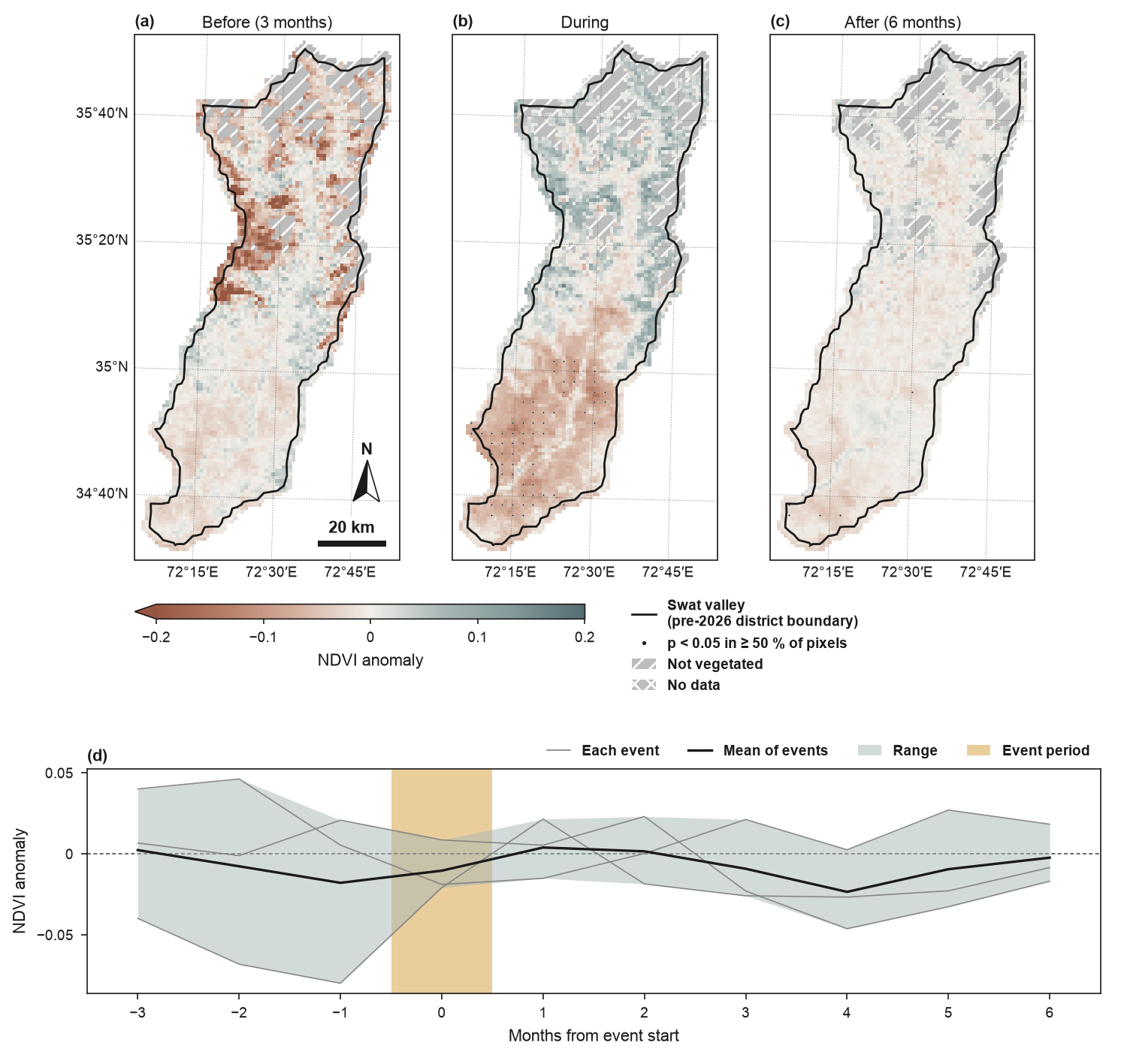
NDVI anomalies around compound hot-dry months in the Swat valley (pre-2026 district boundary): the former Swat district (before January 2026), now Swat and Bar Swat. Events: May–September months with Swat-mean maximum temperature z ≥ +1 and precipitation z ≤ −1 (TerraClimate, 2001–2021): May 2001, May 2006 and August 2009. Boundaries and names shown do not imply any opinion on the legal status of any country or territory. Full code and downloads: gallery.

Method

1. Events are (start, end) date pairs, or runs of True in a boolean series on the data's time steps. An event whose window (window=(-3, 6): steps before the start and after the end) runs past the record, or overlaps the window of an earlier event, is left out with an EventWarning; fig.eofigs_layout lists the events used and dropped.
2. Detrending (detrend="linear", default): a per-pixel linear trend fitted to the baseline steps is removed first, so a long greening or warming trend does not make late events look milder than early ones.
3. Anomalies are taken from the climatology of the baseline steps: all steps outside every event window (or those within baseline=(start, end)), per calendar month for monthly or 16-day data. kind="zscore" divides by the baseline standard deviation of the month. All of this happens at full resolution.
4. Phase maps: for each event, the mean anomaly over the steps before it (the whole pre-event part of the window), during it and after it; the maps show the mean over events, with one shared, symmetric colour scale.
5. Significance across events per pixel: a one-sample t-test of the event means against zero (test="ttest", at least 3 events), or test="wilcoxon" (a two-sided Wilcoxon test at 0.05 can only reach significance with at least 6 events). Dots (or hatching) mark cells of about 1.6 mm where at least half of the pixels are significant, as in trend_map. With fewer than 5 events the test has little power, and the caption says so: the absence of dots does not show the absence of an effect. The tests are not adjusted for multiple comparisons, and the caption says that too: at p < 0.05 about 5 % of the pixels without an effect are marked by chance, in patches where neighbouring pixels are correlated (Wilks 2016; see What the dots mean). fdr="bh" applies Benjamini–Hochberg false discovery rate control at fdr_q (default 2 × alpha), separately to each map, over its valid pixels; the record gives the count of tests and the equivalent p threshold for each map (fig.eofigs_layout["phases"][phase]["fdr"]). See False discovery rate control.
6. Masked classes as in trend_map: grey with diagonal hatching for not vegetated (vegetation indices with a record mean below 0.1), grey with cross-hatching for no data. Pixels without any value in the record lie outside the data and are left white. Other variables have no exclusion unless you pass a boolean grid as exclude= with an exclude_label.
7. Series: the study-area mean anomaly for each event (thin grey), their mean (black) and their spread (interquartile range, or the range with fewer than 4 events). Shading marks the event period: darker up to the length of the shortest event (all events ongoing) and lighter up to the longest (some events ongoing); with events of one length there is a single shade.

The maps carry the phase as a title ("Before (3 months)", "During", "After (6 months)"). With set_style(..., panel_titles=False) they carry only their letters, and the caption sentence names them in order: "(a) before, 3 months; (b) during; (c) after, 6 months; (d) composite series".

Choosing events and windows

The pre-event months of an early-season event can fall in the snow season, when NDVI over snow, cloud and frozen ground is noisy and its anomalies say little about vegetation. In the Swat composite the "before" window of the May events covers February to April, and the "before" map shows patches in the central valley that are not significant. Where this matters, use kind="zscore" so that noisy months weigh less, or choose events and windows that stay within the growing season (for example a shorter window=(-1, 6), or events from June onwards).

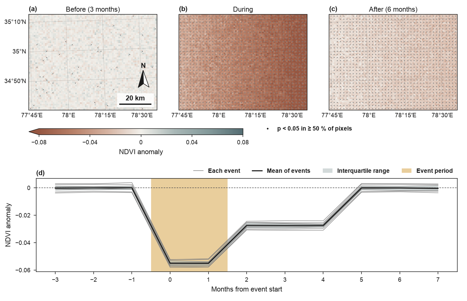
With eight synthetic events the t-test marks the response during and after the events; the maps before the events show only the scattered false positives expected at p < 0.05.

The Swat events

docs/scripts/build_swat_events.py derives the events from TerraClimate (monthly, about 4 km; Abatzoglou et al. 2018, CC0 1.0, through the Microsoft Planetary Computer):

• Swat-mean monthly maximum temperature and precipitation 2001–2021 (the cells whose centres lie inside the outline), as z-scores per calendar month;
• event months: May–September months with tmax z ≥ +1 and precipitation z ≤ −1; consecutive months form one event (with fewer than 3 events the thresholds would be relaxed to 0.75; here they were not);
• the tables are swat_terraclimate_monthly.csv and swat_hot_dry_events.csv in docs/data/swat/.

The NDVI series is the monthly median of MODIS MOD13A1 v6.1 16-day composites (pixel reliability 0–1), averaged to 1 km, 2001–2021 to match TerraClimate.