Trend maps

trend_map draws per-pixel trends with zero-centred colours and significance marks at a size the printed page can show.

import eofigs

eofigs.set_style("elsevier")
fig = eofigs.trend_map(
    ndvi_cube,  # time, y, x with a CRS
    aoi="swat_boundary.geojson",
    aoi_label="Swat valley\n(pre-2026 district boundary)",
)
print(fig.eofigs_layout["caption"])  # the caption sentences on limits, dots and grey
eofigs.save_figure(fig, "figures/fig2")

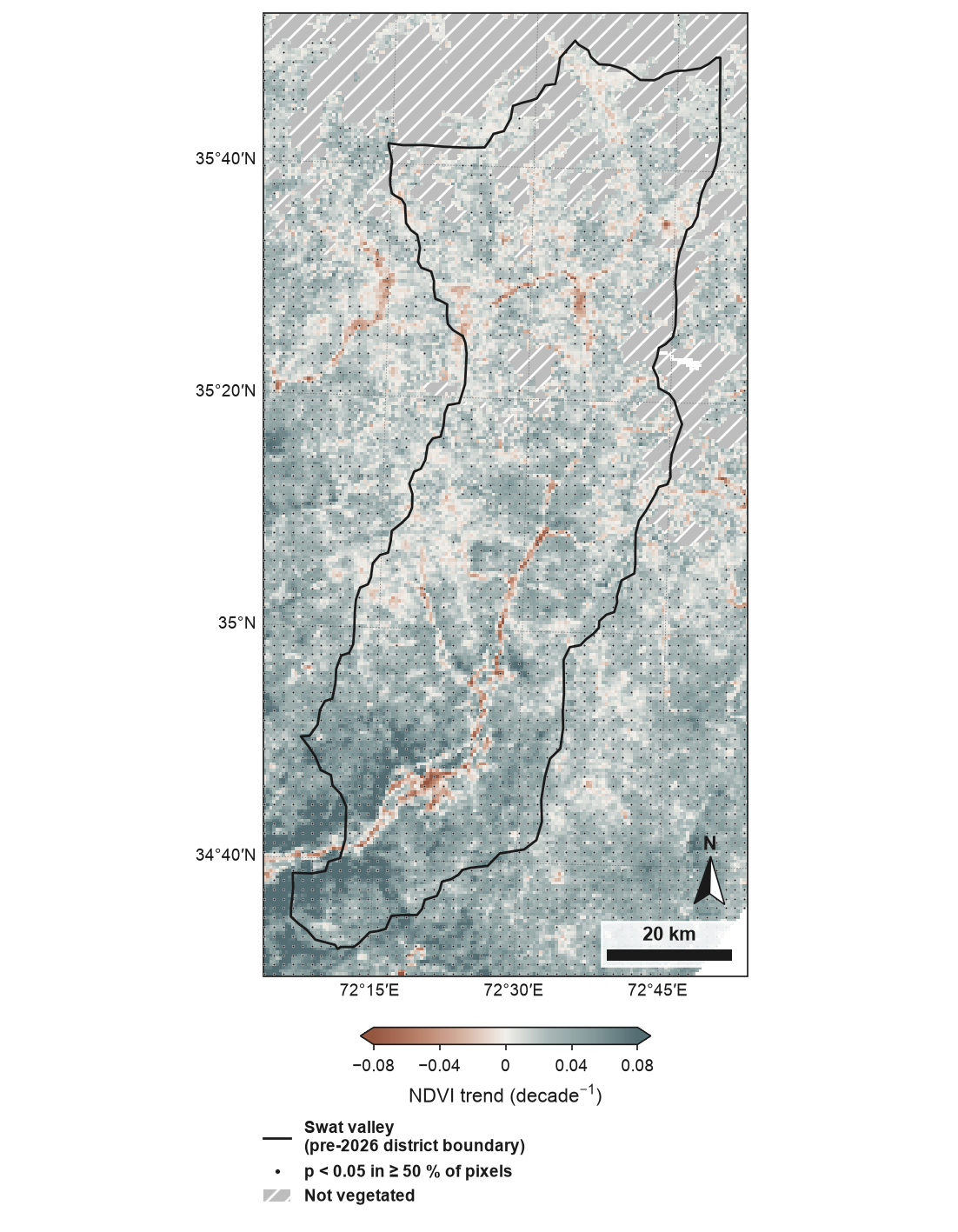
Theil–Sen trend of growing-season NDVI (MODIS MOD13A1, 500 m, May–September median), 2001–2024, around the Swat valley (pre-2026 district boundary): the former Swat district (before January 2026), now Swat and Bar Swat. Colours are limited to ±0.08 decade⁻¹ (98th percentile of |slope|); 1.9 % of pixels exceed this. Dots: at least 50 % of 500 m pixels significant (Mann–Kendall, p < 0.05). Per-pixel Mann–Kendall tests assume serial independence and are not adjusted for multiple comparisons. Grey with diagonal hatching: mean NDVI below 0.1 over the record (not vegetated; 14.9 % of pixels). Boundaries and names shown do not imply any opinion on the legal status of any country or territory. Full code and downloads: gallery.

How it works

1. The trend is computed at full resolution with trend (Theil–Sen slope, Mann–Kendall test), or taken from slope= and pvalue= grids.
2. Then it is reduced to print size: slopes are averaged to the printed pixels; p-values are never averaged.
3. Significance at print size. The map is divided into cells of about 1.6 mm (dot_spacing_mm). A cell gets a dot (or hatching with stipple="hatch") when at least half (sig_fraction) of its valid full-resolution pixels are significant. Dots are 0.35 mm, dark with a thin white edge, so they read on both ends of the colour map.
4. Colours come from the variable library and are centred exactly on zero. Vegetation variables (indices, productivity and structure) use terracotta (browning, loss) to slate teal (greening, gain); other variables use vik in the physically sensible direction (see Variables). The limits are symmetric, at the 98th percentile of |slope| rounded up (limits=), with arrows on the colour bar when values are clipped.
5. Two masked classes in grey #BDBDBD, told apart by hatching (plain grey would be too close to weak greening for colour-blind readers):
6. not vegetated (diagonal hatching): for vegetation indices, pixels whose mean over the record is below 0.1 (rock, snow, ice) are left out (exclude=);
7. no valid trend (cross-hatching): too few valid observations.

Each class has its own legend entry and caption clause with its share of pixels, and is left out when it has none. Pixels without any value in data lie outside the data: they stay white and are not counted in the shares.

The caption sentence

Journals expect the caption to say when colours are clipped. trend_map writes it with the exact numbers:

fig.eofigs_layout["caption"]
# 'Colours are limited to ±0.08 decade⁻¹ (98th percentile of |slope|); 1.9 % of pixels
#  exceed this. Dots: at least 50 % of 500 m pixels significant (Mann–Kendall, p < 0.05).
#  Per-pixel Mann–Kendall tests assume serial independence and are not adjusted for
#  multiple comparisons. Grey with diagonal hatching: mean NDVI below 0.1 over the record
#  (not vegetated; 14.9 % of pixels).'

fig.eofigs_layout also records the limits, the clipped share, the share of significant pixels, the shares of not-vegetated and no-data pixels, the number of marks and the cell size.

What the dots mean

Each pixel is tested on its own. The Mann–Kendall test assumes that the values of a pixel are serially independent; positive autocorrelation (common in vegetation and climate series) makes it reject too often. And with thousands of pixels tested at p < 0.05, about 5 % of the pixels without any trend are marked by chance. Requiring half of the pixels in a cell to be significant thins out isolated false positives, but it is not a correction for multiple testing: neighbouring pixels are correlated, so false positives come in patches. The caption says both. With your own p-values (slope=, pvalue=) eofigs does not know the test, so the caption says only what eofigs did: "Significance from the supplied p-values (alpha = 0.05); eofigs applied no adjustment for multiple comparisons." Wilks (2016) explains why maps of per-pixel significance overstate results and recommends controlling the false discovery rate instead.

False discovery rate control

fdr="bh" applies Benjamini–Hochberg false discovery rate (FDR) control before the marks are drawn:

fig = eofigs.trend_map(ndvi_cube, fdr="bh")  # q = 2 × alpha = 0.10
fig = eofigs.trend_map(ndvi_cube, fdr="bh", fdr_q=0.05)
fig.eofigs_layout["fdr"]
# {'method': 'bh', 'q': 0.1, 'n_tests': 43109, 'n_rejected': 26436, 'p_threshold': 0.0607}

• What it controls: the expected share of false discoveries among the pixels marked significant is at most q. Without it, about 5 % of the pixels without a trend are marked at p < 0.05, however few pixels have a trend.
• q: fdr_q, by default 2 × alpha. Wilks (2016) recommends q = 2 × alpha for spatially correlated fields, for example 0.10 for a field test at 0.05. The legend and the caption give the q used.
• The family of tests is every valid pixel of the grid passed in (finite slope and p-value, not excluded): fig.eofigs_layout["fdr"]["n_tests"]. To make the study area the family, clip the data to it before calling.
• The equivalent p threshold (p_threshold, the largest p-value still significant) is in the record and the caption. It depends on the data: where few pixels have a trend it is far below 0.05; where most have one, it can be above 0.05.
• The rule of marking a cell when at least half of its pixels are significant is unchanged.
• eofigs.stats.fdr_mask does the same for your own figures and analyses.

A field with few trends

A synthetic field with a known answer (the gallery figure): 20 annual NDVI values for 48 × 64 pixels, a trend of 0.04 per decade in a disc of 317 pixels (10.3 %) and none in the other 2 755, noise 0.02.

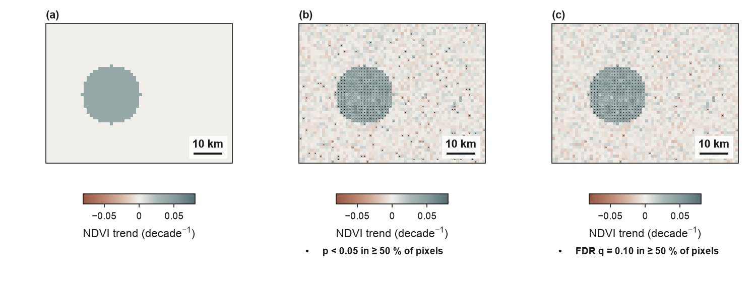
Rule	Pixels marked	With a trend	Without a trend	False share of the marks
p < 0.05	445	314 of 317	131 of 2 755 (4.8 %)	29.4 %
FDR, q = 0.10 (p ≤ 0.010)	330	302 of 317	28 of 2 755 (1.0 %)	8.5 %

With few pixels trending, FDR control is much stricter than p < 0.05: it removes most of the scattered false marks and keeps almost all of the real ones.

A field with many trends

In the Swat NDVI series (the trend map above; 43 109 vegetated pixels with a valid trend) greening is widespread:

Rule	Pixels significant	Equivalent p
p < 0.05	59.3 %	0.05
FDR, q = 0.10	61.3 %	0.061
FDR, q = 0.05	52.4 %	0.026

Here FDR control at q = 0.10 is slightly less strict than p < 0.05, and the maps with and without it look almost the same. This is how the method works, not a fault: it bounds the expected share of false discoveries among the marked pixels (at most 10 %), not the share of trend-free pixels that are marked. When most pixels have a trend, many tests are rejected and the step-up threshold rises. The marks then carry a different guarantee, not a stricter test.

Benjamini, Y., & Hochberg, Y. (1995). Controlling the false discovery rate: a practical and powerful approach to multiple testing. Journal of the Royal Statistical Society: Series B (Methodological), 57(1), 289–300. doi:10.1111/j.2517-6161.1995.tb02031.x

Wilks, D. S. (2016). "The stippling shows statistically significant grid points": how research results are routinely overstated and overinterpreted, and what to do about it. Bulletin of the American Meteorological Society, 97(12), 2263–2273. doi:10.1175/BAMS-D-15-00267.1

Latitude profile

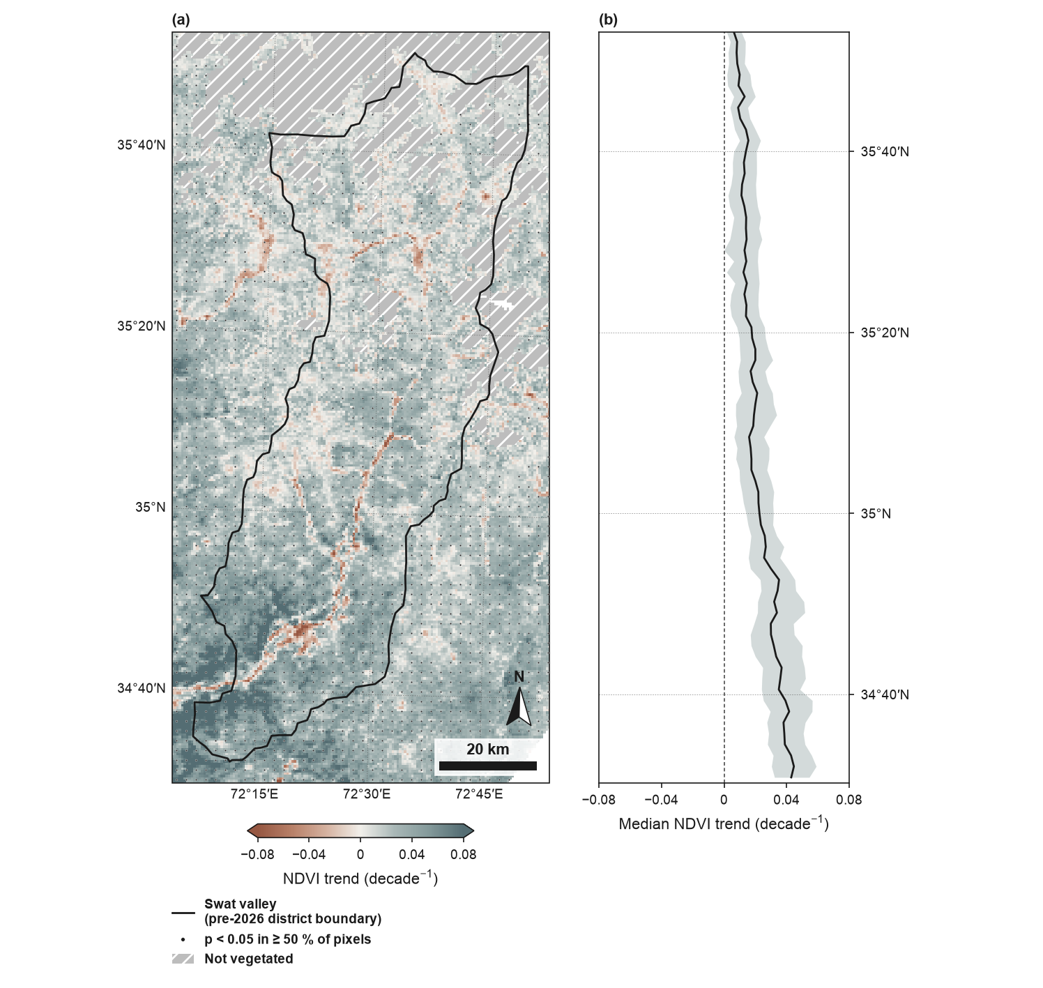
latitude_profile=True adds a panel with the median and interquartile range of the full-resolution slope in latitude bands about 2 mm tall, from valid pixels only; bands with fewer than 20 pixels are skipped. The bands line up with the map.

Inputs

Argument	Use
data	a time-series cube (time, y, x) with a CRS; trend is run on it; pixels without any value lie outside the data and stay white
seasonal, seasonal_correction	seasonal Mann–Kendall test for monthly or other sub-annual data (see Seasonal data)
slope, pvalue	precomputed grids on the same grid and CRS (dimension order may differ); without pvalue there are no marks
alpha, sig_fraction, dot_spacing_mm, stipple	the significance rule and its marks
fdr, fdr_q	Benjamini–Hochberg false discovery rate control of the marks (off by default)
limits	"p98" (default), a number, or None for the largest absolute slope
exclude	"auto", a threshold on the record mean, a boolean grid, or None
aoi	study area outline; the map then shows the study area with a margin
ax, subfigure	draw into existing map axes or into one panel of a larger figure

The Swat NDVI series is in docs/data/swat/, built by docs/scripts/build_swat_ndvi.py from MODIS MOD13A1 v6.1 (NASA LP DAAC, through the Microsoft Planetary Computer); it is not part of the installed package.