Accuracy scatters

accuracy_scatter draws the standard validation figure: estimates against reference values with the 1:1 line, a fitted line and a box of statistics, with labels and units from the variable library.

import eofigs

eofigs.set_style("elsevier")
fig = eofigs.accuracy_scatter(field_agb, predicted_agb, variable="agb")
print(fig.eofigs_layout["stats"])  # every statistic at full precision
print(fig.eofigs_layout["caption"])  # definitions, fitted line, density rule

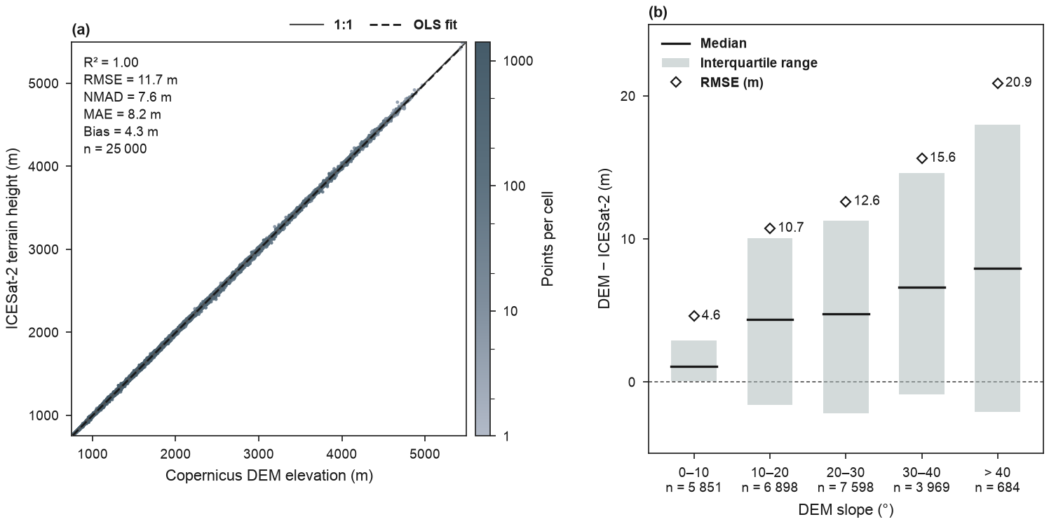
(a) Copernicus DEM GLO-90 elevation against ICESat-2 ATL08 terrain height at 25 000 randomly sampled land segments (2019–2024; strong beams, snow-free, cloud-free, at least 10 terrain photons), converted from the WGS 84 ellipsoid to EGM2008 heights, in the Swat valley (pre-2026 district boundary): the former Swat district (before January 2026), now Swat and Bar Swat. (b) DEM − ICESat-2 by DEM slope class: median, interquartile range and RMSE, with the number of segments per class. Full code and downloads: gallery.

Orientation and fitted line

By default the predicted values go on the x axis and the observed values on the y axis, and the fitted line is the ordinary least-squares regression of observed on predicted. This follows Piñeiro et al. (2008): regressing observed on predicted gives a slope and intercept that describe the model directly (a slope below 1 means the model overestimates high values and underestimates low ones; the intercept shows a constant bias), whereas the reverse regression mixes the model's error into the slope. orientation="observed_x" swaps the axes (the fit then regresses predicted on observed), fit="rma" draws the reduced major axis line, and fit=None leaves the line out.

Piñeiro, G., Perelman, S., Guerschman, J. P., & Paruelo, J. M. (2008). How to evaluate models: Observed vs. predicted or predicted vs. observed? Ecological Modelling, 216(3–4), 316–322. https://doi.org/10.1016/j.ecolmodel.2008.05.006

Pairing the values

The statistics are only as good as the pairing of observed and predicted values. accuracy_scatter pairs them as follows:

Inputs	Paired by
two pandas Series (or DataFrames)	index labels: predicted is put in the order of observed
two xarray DataArrays	coordinates: dimensions and labels put in the order of observed
arrays, or one labelled input and one array	position

Labelled inputs whose labels do not match one to one (labels missing on one side, or repeated) raise an error that counts them, rather than pairing the wrong values; pass .to_numpy() (or .values) to pair by position on purpose. A pandas Series or DataArray of groups is aligned in the same way. fig.eofigs_layout["pairing"] records which rule was used ("index", "coordinates" or "position").

eofigs 0.1.0 paired pandas inputs by position. If you passed two Series whose indexes were in different orders (for example after a merge, a sort or a train/test split), the statistics from 0.1.0 are wrong; re-run with 0.1.1 or later.

Statistics

With observed values O, predicted values P, their means Ō and P̄, and n pairs (pairs with a missing value in either are left out and counted in the record):

Key	Shown as	Formula
r2	R²	squared Pearson correlation of O and P
r	r	Pearson correlation
nse	NSE	Nash–Sutcliffe efficiency, 1 − Σ(P − O)² / Σ(O − Ō)² (it can be negative)
rmse	RMSE	√(Σ(P − O)² / n)
rrmse	rRMSE	100 · RMSE / Ō (%)
nmad	NMAD	1.4826 · median(|e − median(e)|) with e = P − O (Höhle and Höhle 2009)
mae	MAE	Σ|P − O| / n
bias	Bias	Σ(P − O) / n (positive: overestimation)
rbias	rBias	100 · bias / Ō (%)
slope, intercept	Slope, Intercept	of the fitted line, in plot axes (y on x)
n	n	number of pairs

R² is the squared correlation, as most remote sensing validation papers report it; the agreement with the 1:1 line is carried by the RMSE and the bias. The coefficient of determination against the 1:1 line is available as nse, so that a figure never shows a value called R² that can be negative.

The NMAD (normalised median absolute deviation) is the robust spread of the errors that DEM validation usually reports next to the RMSE: for normally distributed errors it equals their standard deviation, and a few blunders barely change it, while they inflate the RMSE.

Höhle, J., & Höhle, M. (2009). Accuracy assessment of digital elevation models by means of robust statistical methods. ISPRS Journal of Photogrammetry and Remote Sensing, 64(4), 398–406. https://doi.org/10.1016/j.isprsjprs.2009.02.003

Numbers in the box carry three significant digits, the statistics with units share one number of decimals, R², r, NSE and the slope get two decimals and the percentages one. Every statistic is kept at full precision in fig.eofigs_layout["stats"] (and per group in ["groups"]), for tables.

Points, groups and density

• Up to 1 000 pairs: open circles. With groups= (up to 6 categories), each group gets an Okabe-Ito colour and its own marker, and the caption lists R² and RMSE for each group.
• Above 1 000 pairs (density="auto"), each point is coloured by the number of points in its cell of a 60 × 60 grid over the axis range, on a log scale, with the densest points drawn on top. The points are rasterised inside vector PDFs, while the axes and text stay vector.
• Both axes share the same limits and ticks, and the plot is square. The statistics box goes in the corner with the fewest points (or stats_loc=).

Several panels

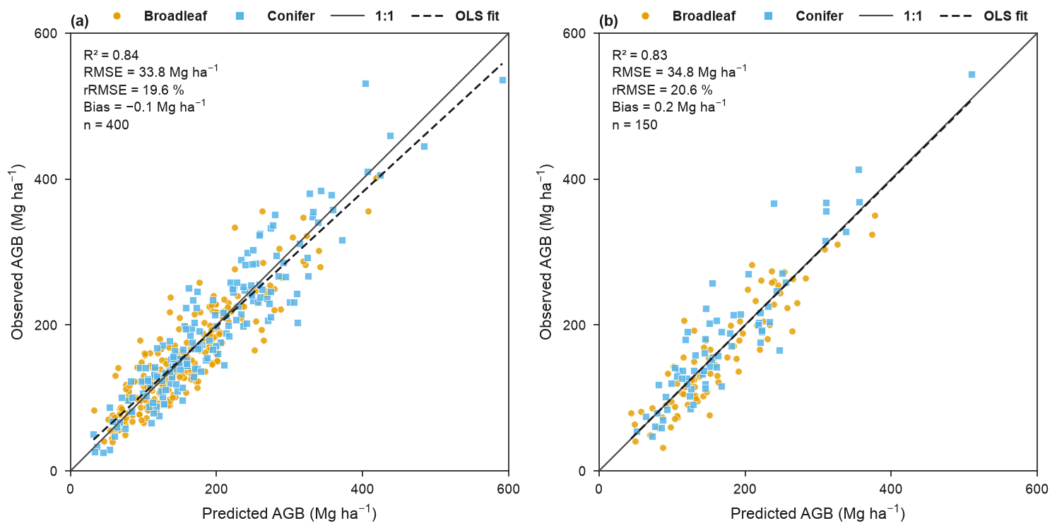
Pass ax= to draw one panel of a larger figure, for example calibration and validation:

fig, axes = eofigs.new_figure("double", ncols=2, height_mm=95)
eofigs.accuracy_scatter(obs_cal, pred_cal, variable="agb", ax=axes[0], labels=["(a)"])
eofigs.accuracy_scatter(obs_val, pred_val, variable="agb", ax=axes[1], labels=["(b)"])

The Swat ICESat-2 pairs

docs/scripts/build_swat_icesat2.py builds swat_icesat2_atl08_dem.csv in docs/data/swat/:

• ICESat-2 ATL08 version 7 land segments (100 m) from 2019 to 2024, cut to the Swat box on NASA's servers with Harmony (a free NASA Earthdata login is needed to run the script);
• a quality rule that does not depend on slope: strong beams, valid best-fit terrain heights, snow-free land (segment_snowcover = 1), no cloud or blowing-snow layer (multiple-scattering warning msw_flag = 0), at least 10 terrain photons per segment, and segment centres inside the Swat outline;
• gross blunders (DEM and ICESat-2 more than 150 m apart) are dropped and counted: there are none, so all 27 619 segments that pass the rule are kept;
• a random subsample of 25 000 of them (seed 2019) is stored, to keep the file under 2 MB; every statistic in the gallery figure is computed from this sample;
• vertical datum: ATL08 heights are above the WGS 84 ellipsoid and the Copernicus DEM is referenced to the EGM2008 geoid; the ATL08 heights are converted to EGM2008 heights with PROJ and NGA's EGM2008 grid before the comparison (the geoid undulation over Swat is about −27 to −39 m, so skipping this step would add a bias of that size);
• the DEM elevation and slope are interpolated bilinearly at each segment centre.

The rule deliberately leaves out the ATL08 terrain height uncertainty (h_te_uncertainty): it grows with the slope within a segment, so a limit on it acts as a slope filter. A 5 m limit, for example, keeps 2 124 segments with a median DEM slope of 1° (against 26° over the whole valley) and an RMSE of 4.2 m, an optimistic picture of the DEM's accuracy in mountains. The stored sample keeps the steep terrain (median slope 20°).

The minimum number of terrain photons has a similar, weaker effect, because steep and forested segments return fewer ground photons. With the other rules applied (strong beams, snow-free, msw_flag = 0, inside the outline, DEM values available):

Minimum terrain photons	Segments	Median DEM slope
none	30 797	20.4°
10 (used)	27 619	19.6°
30	17 013	15.8°
50	10 476	11.0°

A minimum of 10 drops the sparsest terrain fits while keeping the slope mix of the valley; stricter minimums again favour gentle slopes.

Over a 4 km elevation range, metre-level differences are invisible in a scatter: the points lie on the 1:1 line and R² rounds to 1.00, so panel (b) shows the errors themselves. In the sample the DEM is on average 4.3 m above ICESat-2 (RMSE 11.7 m, NMAD 7.6 m). The median difference grows from 1.1 m below 10° to 7.9 m above 40°, and the RMSE from 4.6 m to 20.9 m.