Accuracy scatter: ICESat-2 against a DEM

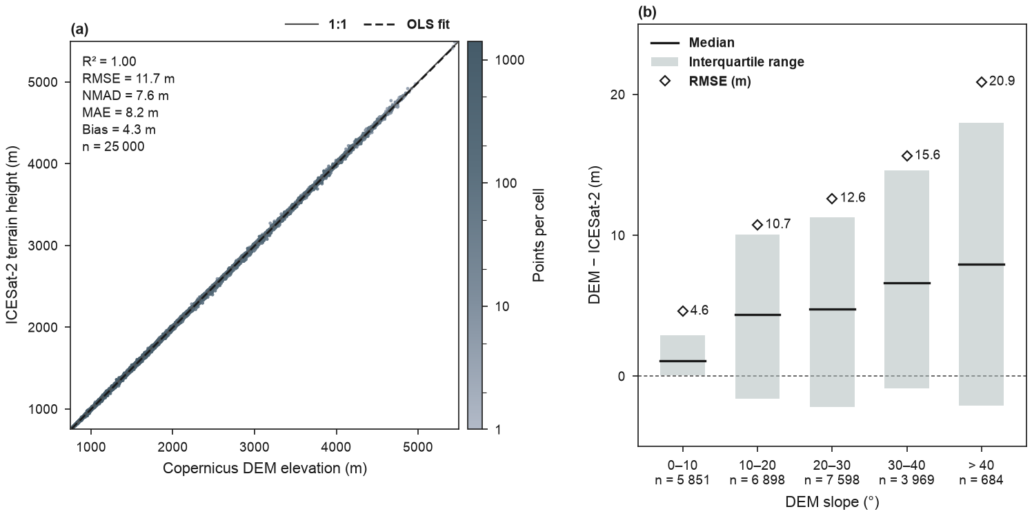
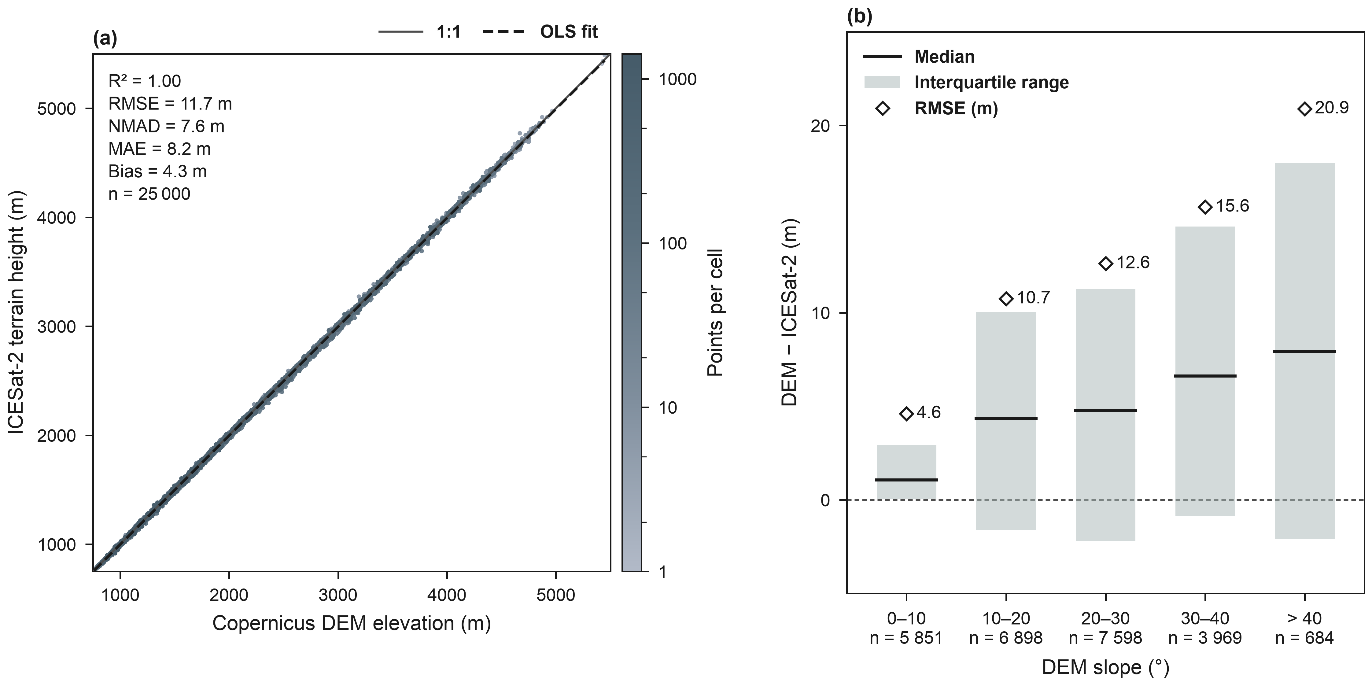
(a) Copernicus DEM GLO-90 elevation against ICESat-2 terrain height at 25 000 ATL08 version 7 land segments (100 m, 2019–2024) in the Swat valley (pre-2026 district boundary): the former Swat district (before January 2026), now Swat and Bar Swat (geoBoundaries). Segments kept: strong beams, a valid best-fit terrain height, snow-free land, no cloud or blowing-snow layer (multiple-scattering warning flag 0), at least 10 terrain photons and a centre inside the outline; no segment differed from the DEM by more than 150 m, so no blunders were dropped. The 25 000 segments are a random subsample (seed 2019) of the 27 619 that passed, and every statistic is computed from this sample. ATL08 heights, given above the WGS 84 ellipsoid, are converted to EGM2008 heights, the datum of the Copernicus DEM, with PROJ and NGA's EGM2008 grid; DEM values are interpolated bilinearly at the segment centres. Point colours show the density of segments; errors and the bias are DEM − ICESat-2, and NMAD is the normalised median absolute deviation of the errors (Höhle and Höhle 2009). (b) The same errors grouped by the DEM slope at the segment centre: median (line) and interquartile range (bar) and RMSE (diamond, value in metres), with the number of segments of each class below its name. The median error and the interquartile range increase from the gentlest to the steepest class. The pairs are docs/data/swat/swat_icesat2_atl08_dem.csv, built by docs/scripts/build_swat_icesat2.py. ICESat-2: ATLAS/ICESat-2 L3A Land and Vegetation Height, Version 7 (NASA NSIDC DAAC, doi:10.5067/ATLAS/ATL08.007). Produced using Copernicus WorldDEM™-90 © DLR e.V. 2010-2014 and © Airbus Defence and Space GmbH 2014-2018 provided under COPERNICUS by the European Union and ESA; all rights reserved.

Script PDF PNG, 600 dpi

from pathlib import Path

import matplotlib as mpl
import numpy as np
import pandas as pd
from matplotlib.lines import Line2D
from matplotlib.patches import Patch

import eofigs

DATA = Path(__file__).resolve().parents[1] / "docs" / "data" / "swat"
SLOPE_CLASSES = [0, 10, 20, 30, 40, 90]
CLASS_NAMES = ["0–10", "10–20", "20–30", "30–40", "> 40"]
IQR_COLOUR = eofigs.palettes.terra_slate[4]  # the light teal of the envelope bands
TEXT = "#1A1A1A"

pairs = pd.read_csv(DATA / "swat_icesat2_atl08_dem.csv")
error = pairs["dem_elevation_m"] - pairs["icesat2_height_egm2008_m"]
slope_class = pd.cut(pairs["dem_slope_deg"], SLOPE_CLASSES, right=False, labels=CLASS_NAMES)
by_class = error.groupby(slope_class, observed=False).agg(
    n="size",
    median="median",
    q25=lambda e: e.quantile(0.25),
    q75=lambda e: e.quantile(0.75),
    rmse=lambda e: np.sqrt(np.mean(e**2)),
)

eofigs.set_style("elsevier")
fig, (scatter, classes) = eofigs.new_figure("double", ncols=2, height_mm=95)
fig.get_layout_engine().set(wspace=0.08)  # room between the colour bar and panel (b)
eofigs.accuracy_scatter(
    pairs["icesat2_height_egm2008_m"],
    pairs["dem_elevation_m"],
    variable="elevation",
    stats=("r2", "rmse", "nmad", "mae", "bias", "n"),
    observed_label="ICESat-2 terrain height (m)",
    predicted_label="Copernicus DEM elevation (m)",
    ax=scatter,
    labels=["(a)"],
)

# (b) errors by slope class: interquartile bars and medians, as in the envelope plots
for i, row in enumerate(by_class.itertuples()):
    classes.fill_between([i - 0.3, i + 0.3], row.q25, row.q75, color=IQR_COLOUR, alpha=0.5,
                         linewidth=0)  # fmt: skip
    classes.plot([i - 0.3, i + 0.3], [row.median] * 2, color=TEXT, linewidth=1.2)
    classes.plot(i, row.rmse, marker="D", markersize=3.5, markerfacecolor="white",
                 markeredgecolor=TEXT, markeredgewidth=0.8, linestyle="none")  # fmt: skip
    classes.annotate(f"{row.rmse:.1f}", (i, row.rmse), xytext=(4, 0), textcoords="offset points",
                     va="center", size=mpl.rcParams["xtick.labelsize"])  # fmt: skip
tick_labels = [f"{c}\nn = {n:,}".replace(",", " ") for c, n in by_class["n"].items()]
classes.axhline(0, color="#4D4D4D", linewidth=0.6, linestyle=(0, (3, 2)), zorder=0)
classes.set_xticks(range(len(CLASS_NAMES)), tick_labels)
classes.set_xlim(-0.6, len(CLASS_NAMES) - 0.4)
classes.set_ylim(-5, 25)
classes.set_xlabel("DEM slope (°)")
classes.set_ylabel("DEM − ICESat-2 (m)")
eofigs.tidy_axes(classes)
classes.legend(
    handles=[Line2D([], [], color=TEXT, linewidth=1.2, label="Median"),
             Patch(facecolor=IQR_COLOUR, alpha=0.5, label="Interquartile range"),
             Line2D([], [], marker="D", markersize=3.5, markerfacecolor="white",
                    markeredgecolor=TEXT, markeredgewidth=0.8, linestyle="none",
                    label="RMSE (m)")],
    loc="upper left", frameon=False, borderaxespad=0.6,
    prop={"size": mpl.rcParams["xtick.labelsize"], "weight": "bold"},
)  # fmt: skip
eofigs.label_panels([classes], ["(b)"])


# README card: panel (b), the errors by slope class
readme_card = [classes]

if __name__ == "__main__":
    print(scatter.eofigs_layout["caption"])
    print(by_class.round(2))
    print(eofigs.save_figure(fig, "accuracy_scatter_icesat2"))

Figure check

Figure check (elsevier): passed
  PASS  size: 190.0 x 95.0 mm (double width).
  PASS  resolution: 600 dpi (at least 500 for figures with text and images).
  PASS  font size: Smallest text 7 pt (minimum 7 pt).
  PASS  fonts: Fonts in use: Arial.
  PASS  colour-blind safety: 7 categorical colours, all distinguishable.
  PASS  colour maps: Colour maps: eofigs.slate_density (sequential).